Ian Brown
October 2017
1. Background
In August 2017, we flew a UAV (unmanned aerial vehicle, or drone) over part of the now abandoned Owhiro Bay Quarry, South Wellington, to record high resolution photographs of the excavated slope. This was to provide information to assist the New Zealand Geotechnical Society two day course in Principles and Practice of Engineering Geology.
On September 5, Stuart Read and Fred Baynes led a field exercise logging part of the greywacke quarry slopes (NZ Geotechnical Society field course).
Above the area of the field mapping exercise there is a well defined slope failure affecting one of the intermediate benches of the quarry. As part of a research project, we have been documenting shallow failures in local greywacke rocks, with the objective of carrying out back analysis to get a better understanding of shear strengths along the failure surfaces.
This failure was of interest to us, and we have used the UAV data to build a slope model that we can analyse in 3D. This note explains how we went about that using the computer program TSLOPE.
One of the objectives of the field logging course is to determine the applicable Geological Strength Index (GSI) for the greywacke rock mass. Using our TSLOPE model we have been able to investigate, through back analysis, how GSI might vary at the bench failure.
2. UAV data capture
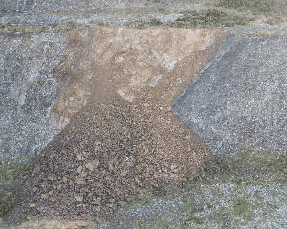
The UAV used to photograph the quarry was a DJI Phantom 4 UAV Pro. A subset (40) of the large number of images were processed using Pix4D software to generate the ortho-mosaic photograph shown in Figure 1. There was good overlap of images over the area, with more than 5 images overlapping for every pixel location.
Figure 1 Photograph from UAV showing area of shallow slope failure
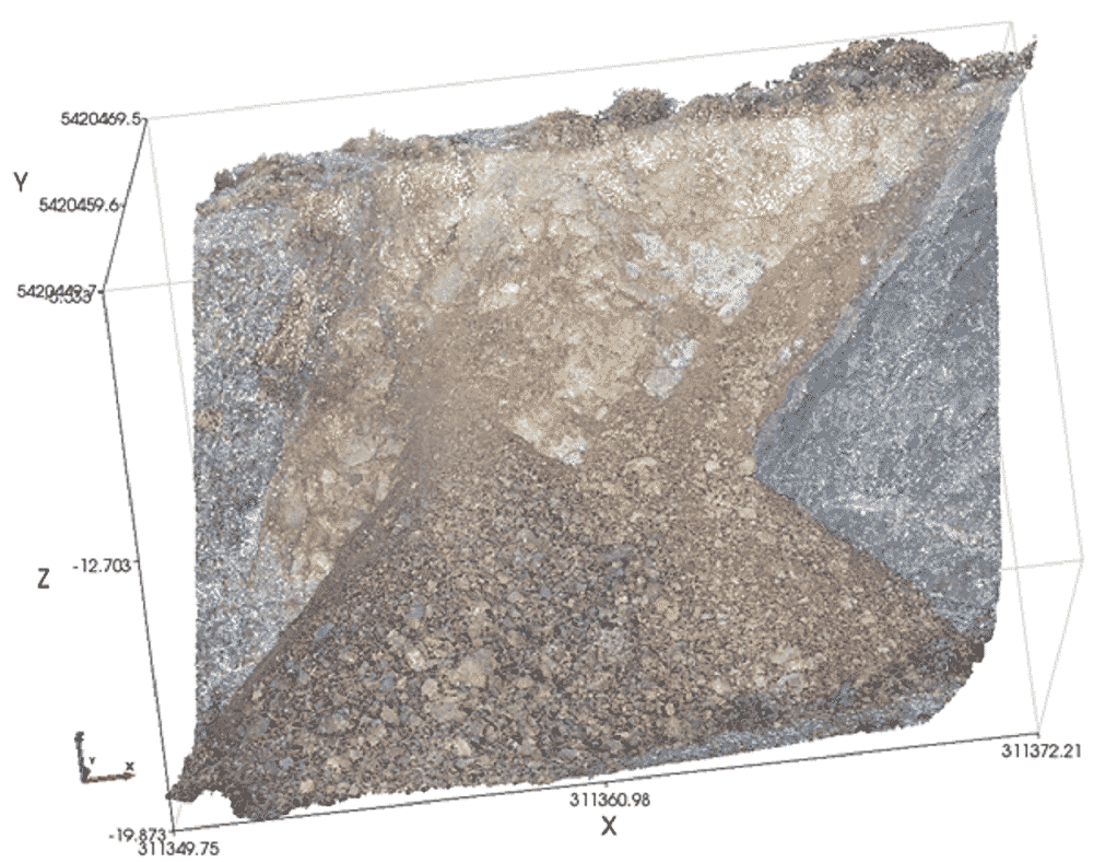
A cloud of points with values for x, y, z as well as RGB (red, green, blue values for each point) was also generated by Pix4D. The cloud of points data (814,802 points) were loaded into TSLOPE to assist with visualisation of the slope, as shown in Figure 2. Because of the RGB attributes of each point, a photo-like image is created.
Figure 2. Cloud of points as displayed in TSLOPE.
3. Site description
The shallow slope failure has occurred on a bench slope on one of the intermediate levels of the quarry. Before closure, the quarry produced aggregate for the local construction industry from a highly indurated quartzofeldspathic sandstone, with interbedded siltstone, known locally as “greywacke”. The rock is variably weathered, as shown by the brown colours in Figures 1 and 2.
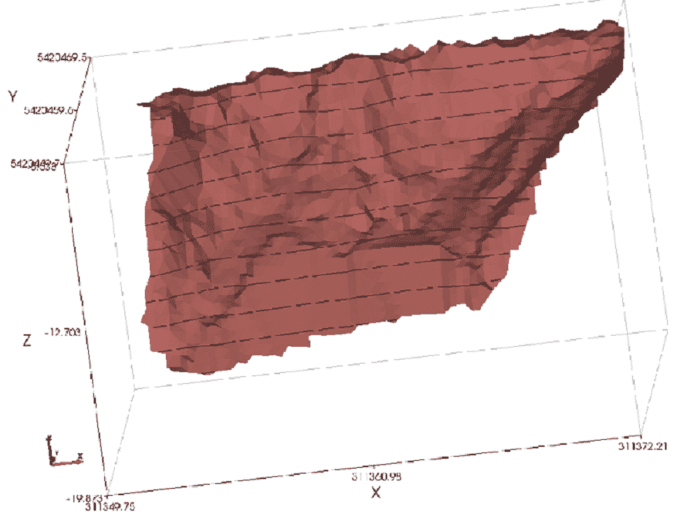
Slope failures in the quarry are controlled by rock structure. As shown on Figures 1 and 2, at the right hand side the failure has occurred along a bedding plane. Well developed joint planes comprise the other part of the failure surface. The composite failure surface is then assumed to continue towards the toe of the slope, where it is covered by debris.
The slope failure has dimensions of about 10m height, and about 15m width at the top of the bench.
4. Surface modelling
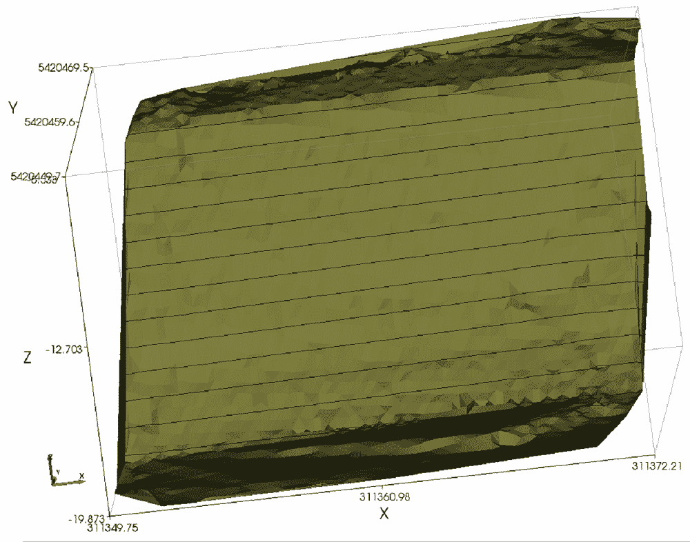
To provide a model that can be used to back calculate in situ strengths that applied at the time of slope failure, we prepared a model of the original topographic surface (Figure 3), and the failure surface (Figure 4).
We used CloudCompare1 software to clean up the cloud of points, and to produce surfaces that could then be transferred to TSLOPE.
Figure 3. Bench surface before slope failure.
Figure 4. Modelled failure surface, note bedding plane on right.
Greywacke material properties were then entered, with unit weight (unsaturated) of 21 kN/m3, Mohr Coulomb parameters – cohesion of 5 kPa, and angle of friction of 35o. These numbers were an estimate, reflecting the low stresses acting on the failure surface.
5. Three dimensional stability analysis
A three dimensional slope case was then defined based on the two surfaces. It was assumed that there were no groundwater pressures acting on the failure surface.
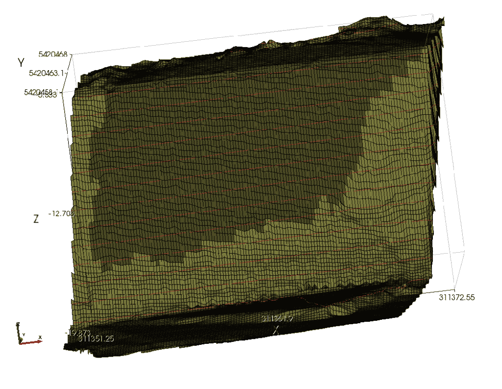
The slope case involved discretising the model into vertical columns overlying the basal surface. There were 200 columns across the width of the model, as shown in Figure 5. Each column is 0.17m wide. The darker colour columns are the active columns involved in the slope stability calculations.
Figure 5. Three dimensional slope stability model showing arrangement of vertical columns.
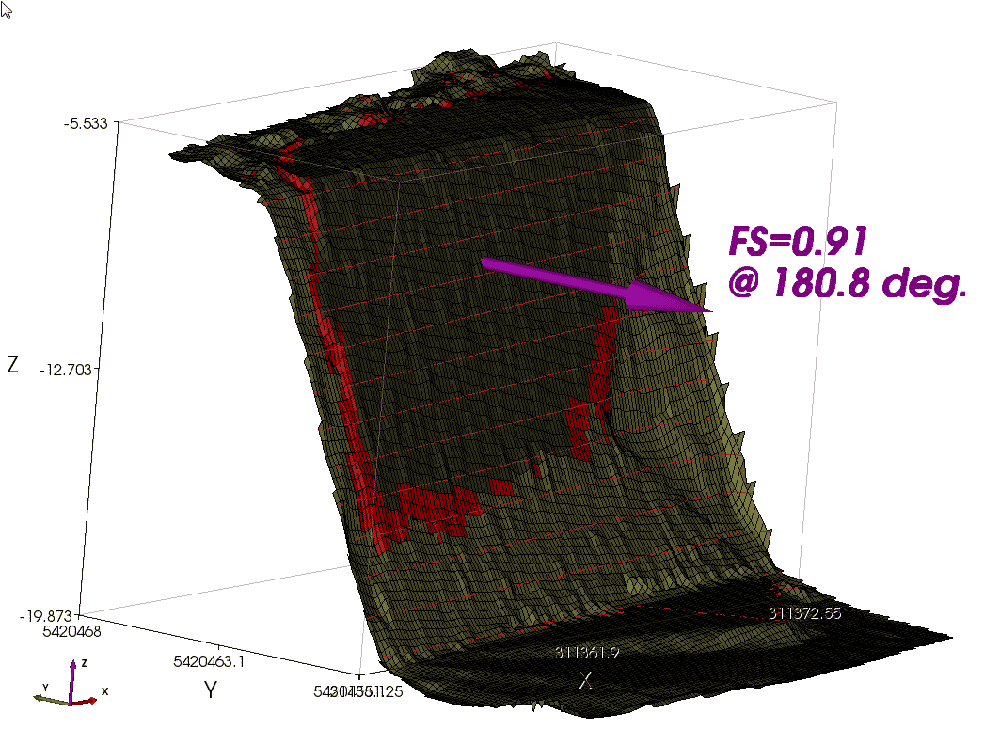
TSLOPE then provided a solution using Spencer’s method, with a calculated factor of safety of 0.91 with failure bearing at 180.8 degrees (Figure 6). This suggests that the strengths used in the model are a little lower than would have applied at the time of failure.
Figure 6. Result of 3D analysis using Spencer’s method.
6. Two dimensional stability analysis
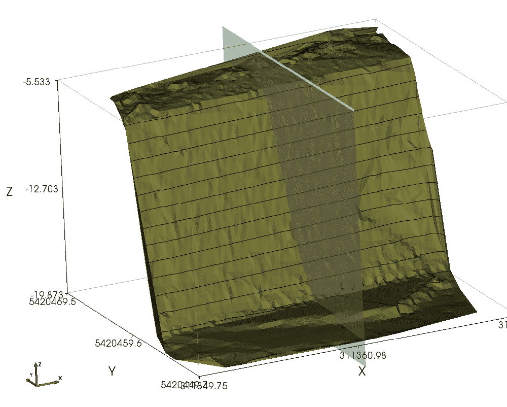
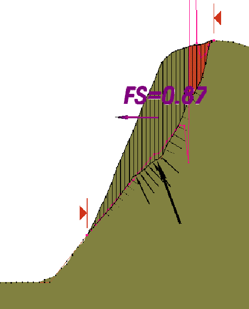
We can locate an arbitrary cross section through the TSLOPE model (Figure 7). The cross section is then used to carry out a conventional 2D slope stability analysis, where the 3D columns become 2D slices (Figure 8).
Note the difference in factors of safety calculated with 3D (0.91) and 2D (0.87).
Figure 7. Cross section location
Figure 8. 2D slope stability analysis using Spencer’s Method
7. Back analysis
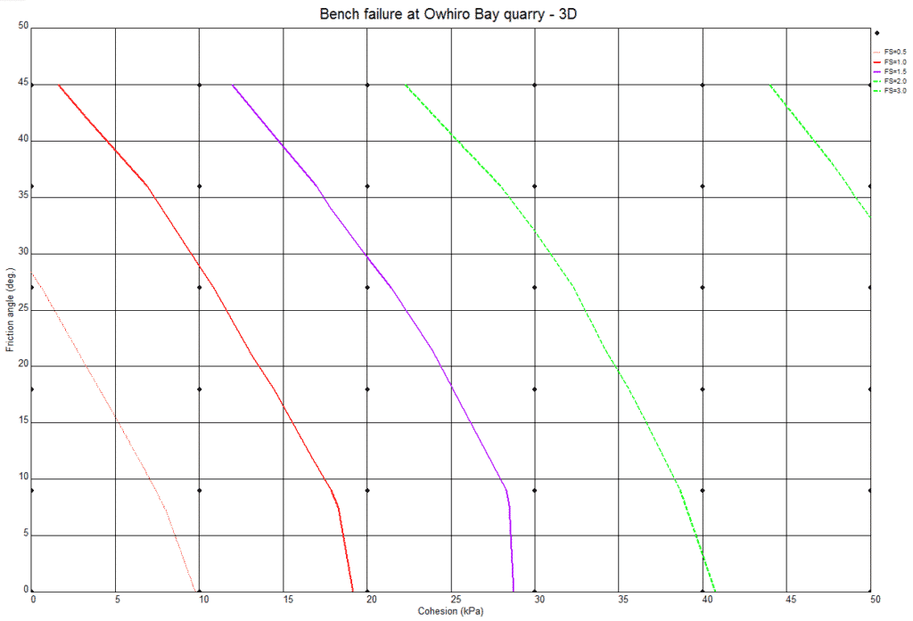
To help understand the range of strengths that would apply at a factor of safety of 1.0, we have carried out a back analysis of the 3D slope model using different combinations of Mohr Coulomb parameters c and phi. A cross plot showing the range of strengths corresponding to different factors of safety is shown in Figure 9.
Figure 9. Cross plot of friction angle (vertical axis) and cohesion with calculated factor of safety. Red line is FS = 1.
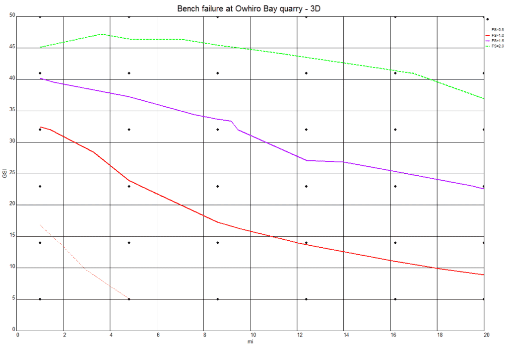
We can change the failure criterion that applies to the failure surface to Generalised Hoek-Brown, and carry out a further back analysis. The Generalised Hoek-Brown criterion is a non linear criterion that is often used for analysis of rock slopes. It requires four parameters; intact uniaxial strength, GSI, disturbance, and mi (material constant for the intact rock).
We can hold two of the variables constant, in this case intact uniaxial strength (3 MPa) and disturbance (0.3), then back calculate the values of GSI and mi to provide a cross plot showing change in factor of safety (Figure 10).
Figure 10. Cross plot of GSI (vertical axis) and mi with calculated factor of safety. Red line is FS = 1.
8. Concluding remarks
To help understand the range of strengths that apply in shallow slope failures, it is recommended that other slope failures are systematically studied in this way. By aggregating cross plots for a number of slopes as shown in Figures 9 and 10, it will be possible to show the range of strengths that apply to shallow weathered greywacke.
We are currently documenting similar slope failures around the Wellington region as part of an ongoing research project. We would like to know about any other slope failures that could be contributed to this study.
The GSI estimates made during the field exercise have not been collated, but we were shown estimates around 40 – 50. This can be compared with the red curve shown on Figure 10 where we might suggest a GSI of 20 – 30 applies at the slope failure.
There could be a number of explanations for a variation in our estimates of GSI. One that could be important is the field mapping was biased towards the small scale structures that were in front of the observers, whereas the slope failure was controlled by larger structures, in this case bedding.
We welcome further discussion on this topic.
