by Ian Brown D.Eng, CPEng
- Background
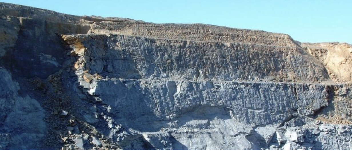
In 1996 a slope failure occurred at the Round Hill open pit mine, operated by Macraes Mining Company Ltd. The failure as shown in Figure 1, involved three benches at an intermediate slope that was being pushed back towards the final high wall location.
Figure 1. Photograph of pit area involved with slope failure.
The slope failure was well documented. We have taken the relevant data, and developed a three dimensional slope model using TSLOPE, an innovative software package for slope stability analysis. TSLOPE is able to carry out 3D limit equilibrium analysis of columns overlying a shear failure surface. The failure surface can be any shape, such as formed by interconnecting fault surfaces as in this open pit mine failure. Stability analyses can also be carried out in 2D, using arbitrary sections drawn across the 3D model.
We show by our study of this open pit mine failure that there can be a significant difference between factors of safety calculated using 3D and 2D analyses.
- Geological structure
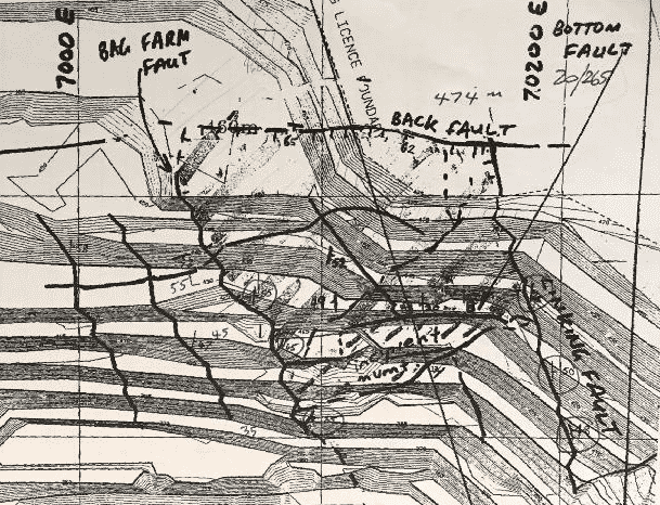
Geological mapping of the pit face showed that the rock mass involved with the failure was bounded by four faults. A geological map of the area was available, as shown on Figure 2.
Figure 2. Geological sketch map of slope failure area.
The four faults that controlled the slope failure are shown. The Bag Farm Fault on the western side dipping to the east; the Back Fault at the top of the slope, dipping south; the Linking Fault on the east side, also dipping east; the base of the slope failure was controlled by the Incipient Fault with a shallow dip to the west.
- Modelling the slope failure surface
TSLOPE relies on the user having access to a software package that is able to model surfaces. In this case, the four fault surfaces were modelled using Leapfrog®, and the surfaces were imported into TSLOPE using the .obj formatted files for each surface. The modelling process enabled us to use the structural information from the geological mapping (dip and dip direction), and follow the outcrop pattern of the faults so that the modelled surfaces reflected the irregularities of the fault surfaces and were not approximated as simple planar surfaces.
- Surfaces in TSLOPE
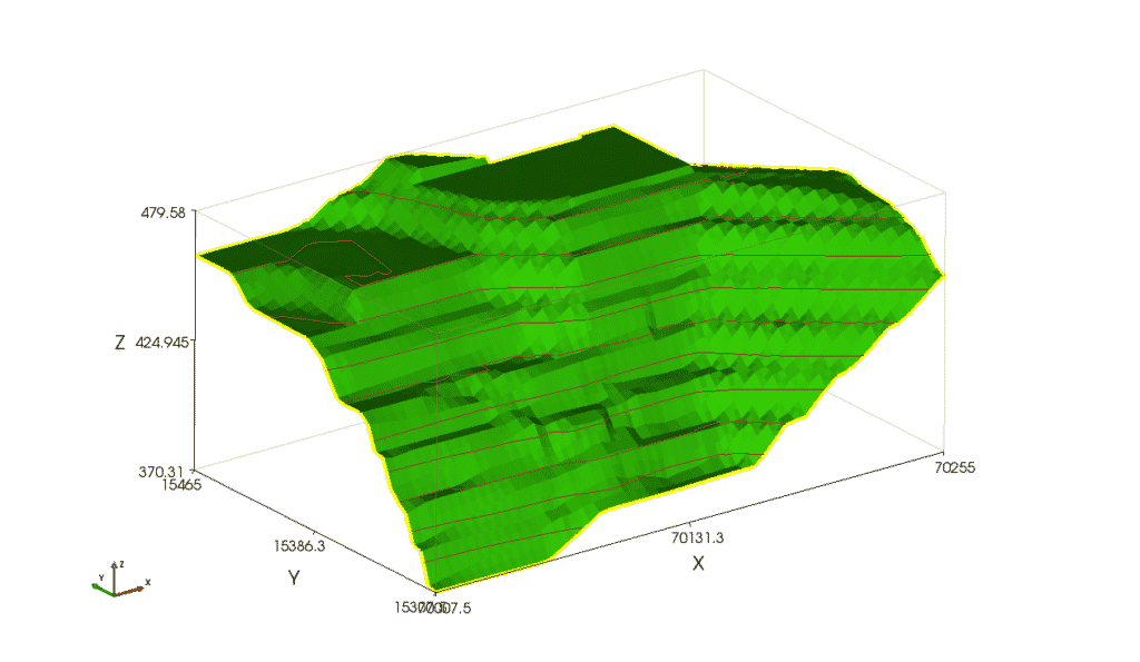
The ground surface prior to slope failure was available as a gridded file with x, y, z coordinates. They were loaded directly into TSLOPE (Figure 3).
Figure 3. Pit slope topography, as modelled in TSLOPE.
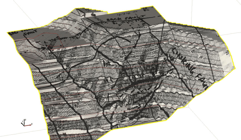
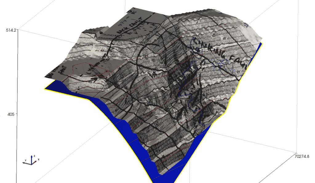
As a check, we draped the surface geology sketch on our model of the pit slope (Figure 4).
Figure 4. Surface geology sketch draped on pit slope.
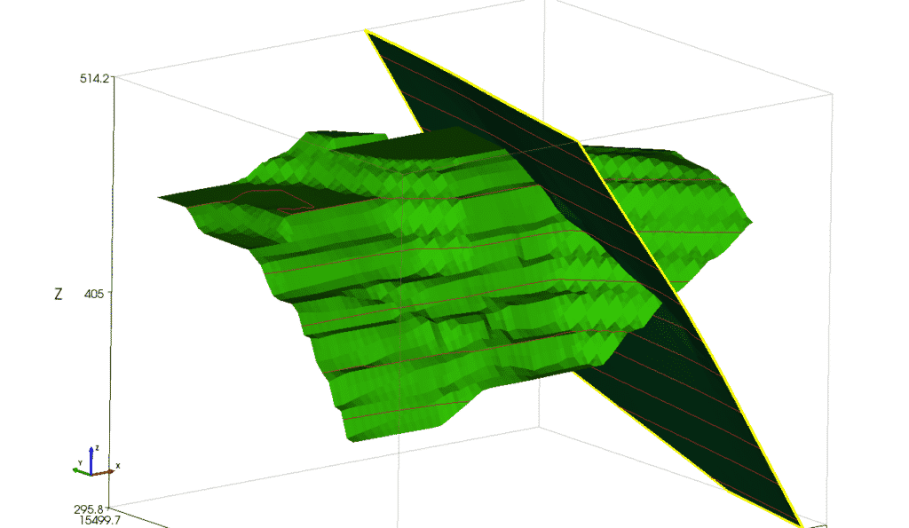
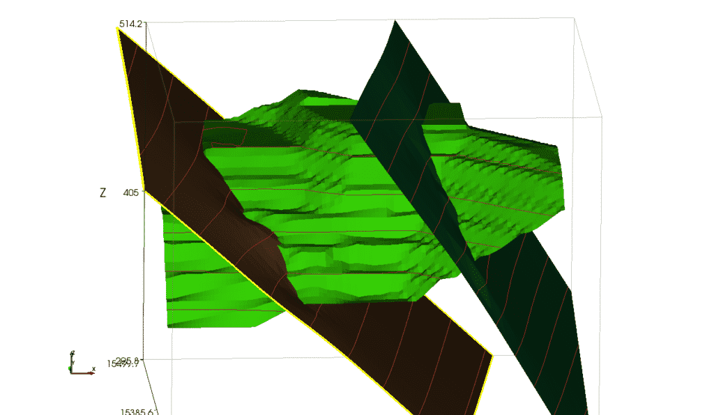
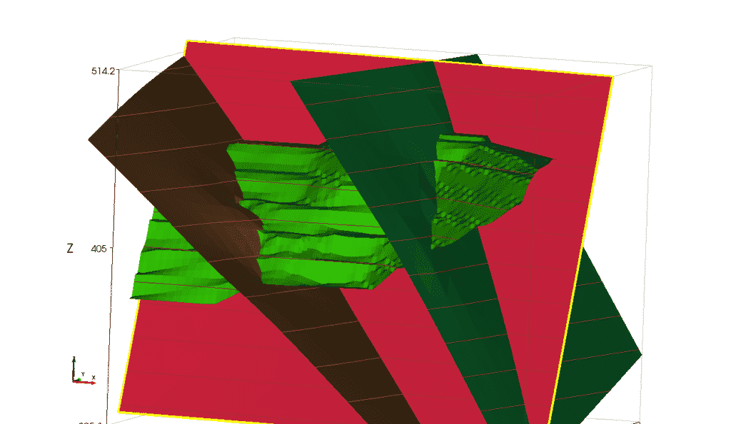
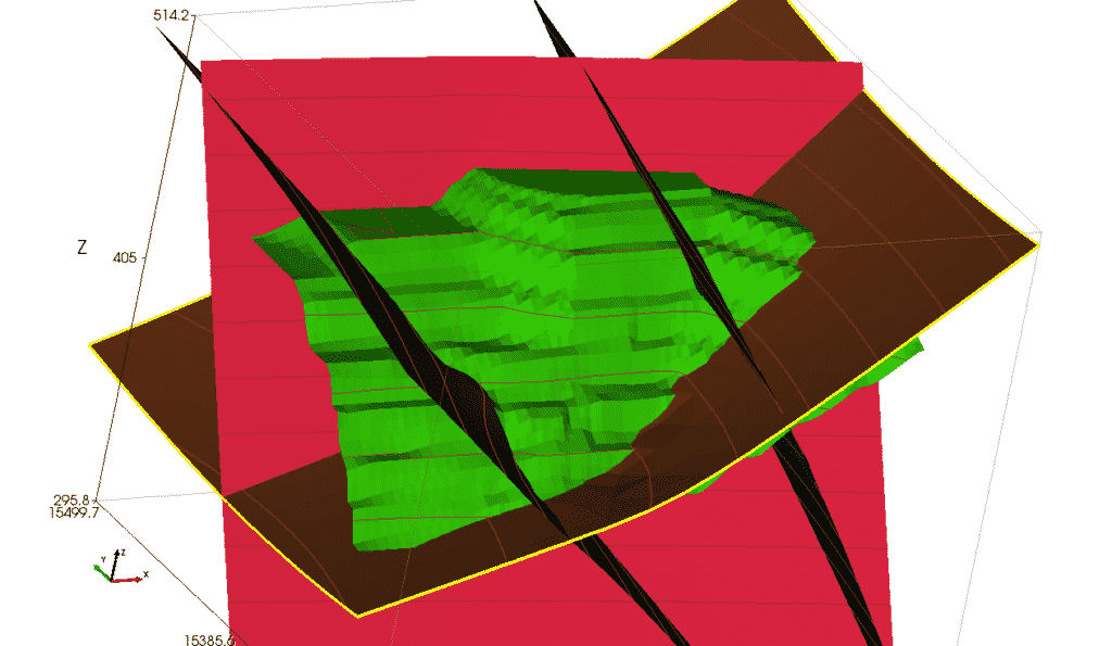
Each fault was loaded into TSLOPE from .obj files. Other formats that are available include .dxf, cloud of points (x, y, z).
The first fault loaded was the Linking Fault (Figure 5) followed by the Bag Farm Fault (Figure 6), the Back Fault (Figure 7), then the Bottom Fault (Figure 8).
Figure 7 Linking Fault.
Figure 8. Bag Farm Fault added.
Figure 9. Back Fault added.
Figure 10. Bottom Fault added.
The final surface added to the TSLOPE model was the phreatic surface, as a modelled surface (x,y,z) (Figure 11).
Figure 11. Phreatic surface added.
TSLOPE has the ability to create composite surfaces by combining any of the surfaces that have been loaded. For this open pit slope, we needed to make a composite failure surface comprising the Back Fault, the Bag Farm Fault, and the Incipient Fault. The fourth fault, the Linking Fault dips east and forms a tension crack rather than a shear failure surface.
In order to correctly model the wedge of rock that underlies the Linking Fault with shearing occurring along the Incipient Fault segment of the composite failure surface, we created a composite topographic surface formed by the pit slope and the foot wall of the Linking Fault.
- Cross sections
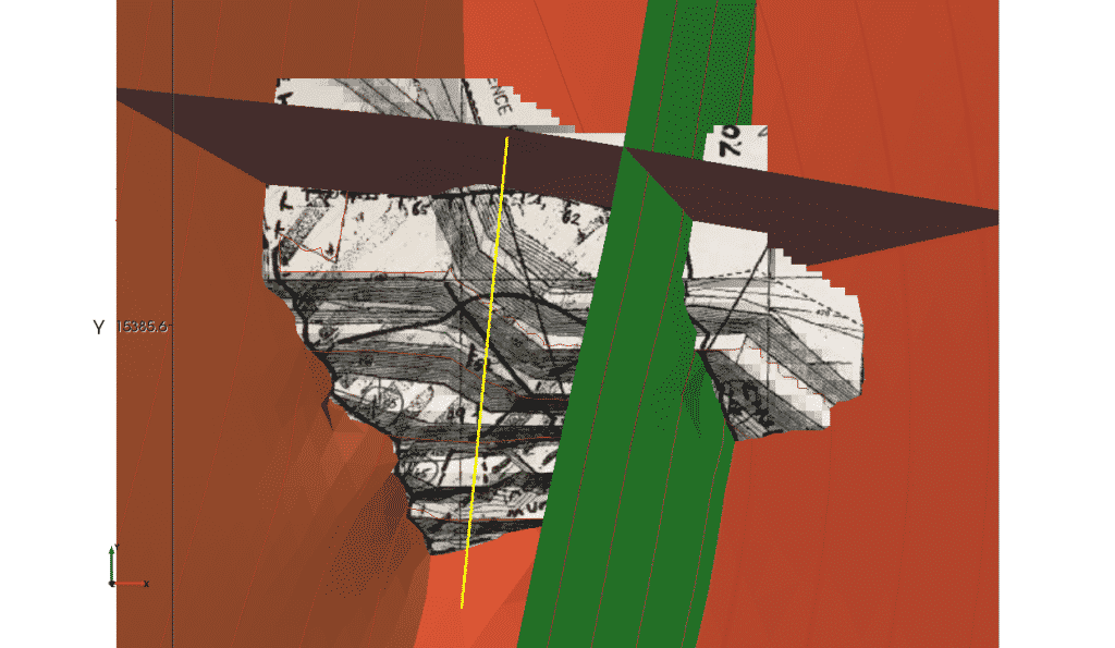
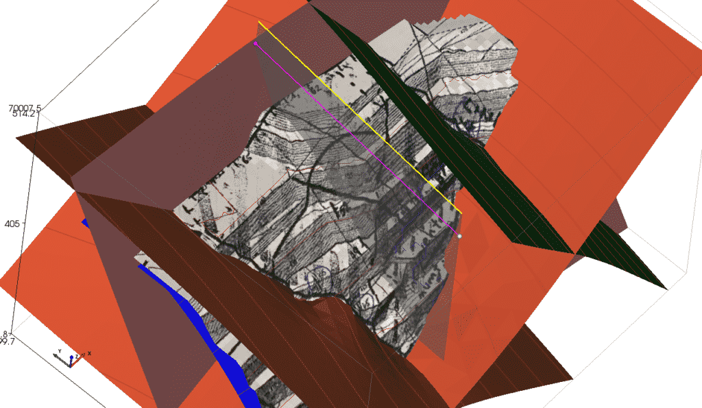
TSLOPE is able to draw arbitrary cross sections through the slope model (Figures 12 & 13).
Figure 12. Cross section plan location shown by yellow line.
Figure 13. Cross section location in perspective view.
- Slope cases
TSLOPE allows the user to set up a number of slope cases based on the slope model and material parameters (density, shear strength). The slope cases may be either 3D, or 2D.
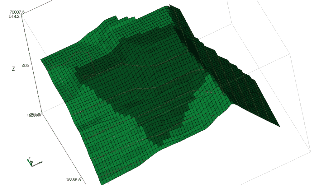
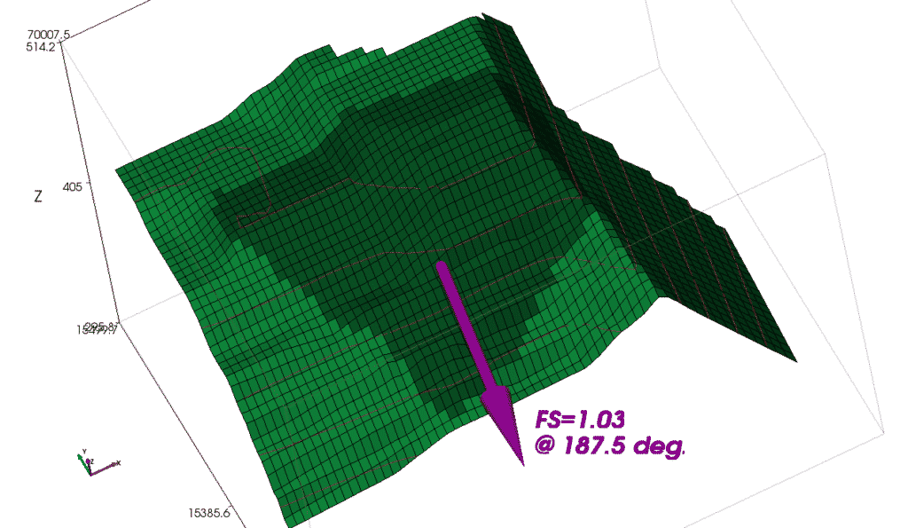
For the open pit slope, we created a 3D slope case using the composite topographic surface, and the composite failure surface as discussed in section 4. The model created was discretised into columns, with the columns taking part in the slope failure shown in a darker shade (Figure 14).
The phreatic surface was also used so that pore water pressures acting on the failure surface were applied to the base of each column (or slice) in the limit equilibrium calculations.
Figure 14. 3D slope model, darker columns are located above composite shear surface.
Using Spencer’s method, the overall factor of safety for the 3D slope case is shown in Figure 15.
Figure 15. Factor of safety, and sliding direction for 3D slope case.
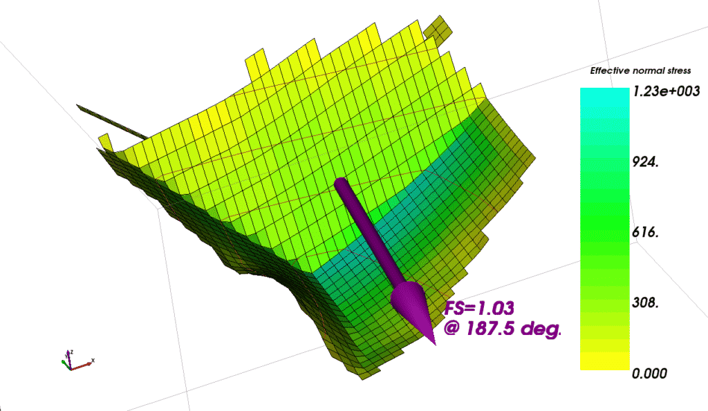
We can visualise the results of our 3D calculations in various ways. The effective normal stresses on the base of each column can be shown (Figure 16).
Figure 16. Effective normal stress at the base of each column.
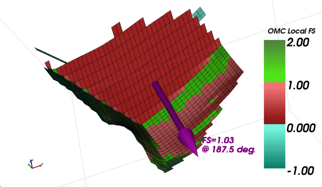
TSLOPE uses the Ordinary Method of Columns, a 3D extension of the Ordinary Method of Slices, as a starting point of the limit equilibrium calculations. This method assumes that each column is independent of its adjacent column, and the driving and resisting forces are calculated at the base of each column. The ratio of these forces gives a local factor of safety which can give insight into slope behaviour (Figure 17).
Figure 17. Local factors of safety calculated using Ordinary Method of Columns.
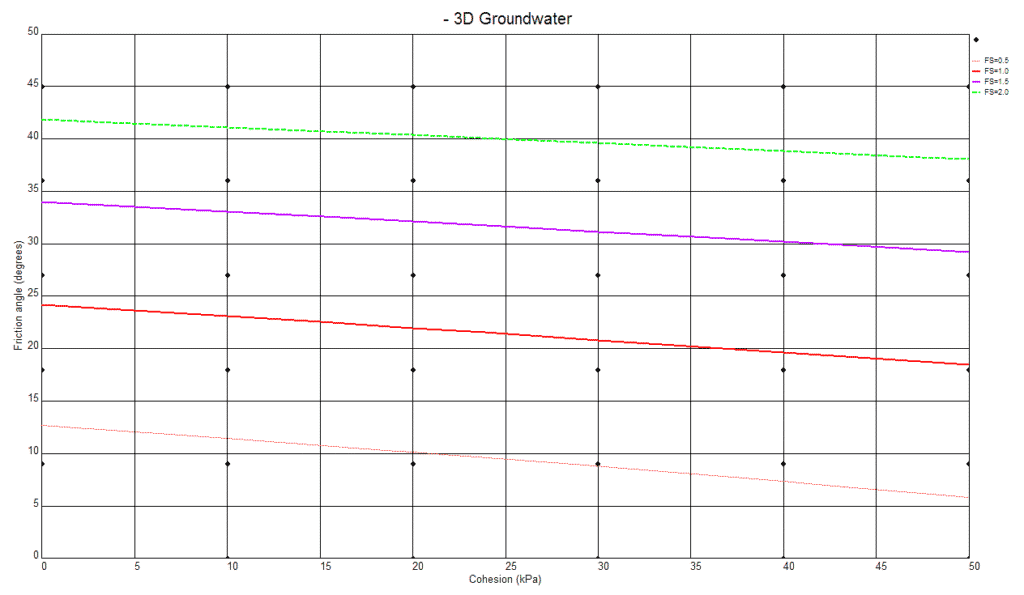
Another analysis that we can carry out with the 3D slope model is a back calculation looking at the change in factor of safety calculated as we vary the shear strength parameters c (cohesion) and phi (angle of friction). The cross plot generated by TSLOPE is shown on Figure 18.
Figure 18. Results of back calculation – 3D slope case
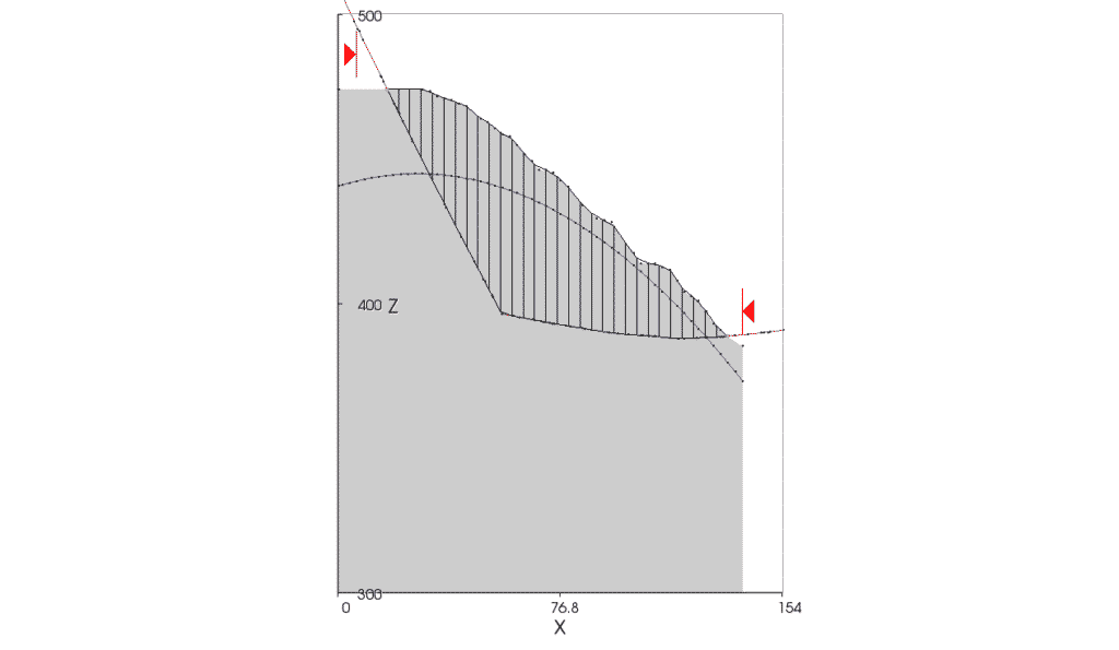
A 2D slope case using the same surfaces as for the 3D slope case was created along the cross section shown in Figures 12 and 13. This slope case divided the section into 2D slices above the failure surface, the equivalent of our 3D columns (Figure 19).
Figure 19. 2D slope case showing slices located above the composite failure surface, at this location comprising the Incipient Fault (shallow dip) and the Back Fault. Phreatic surface shown in blue.
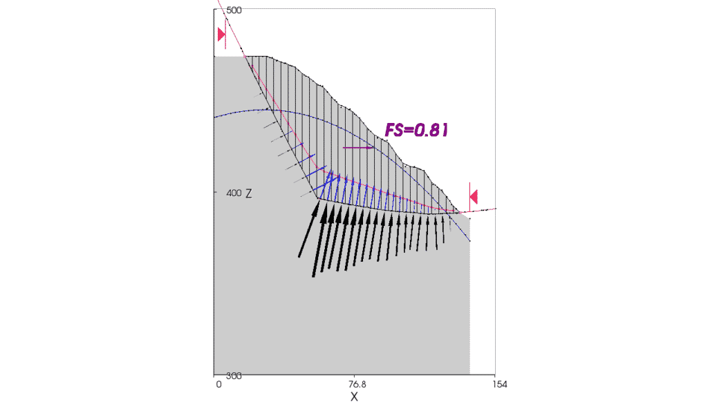
The result of a 2D limit equilibrium analysis of the 2D slope case, using Spencer’s method, is shown in Figure 20.
Figure 20. Result of 2D stability analysis showing line of thrust (red), normal forces (black) and pore pressures (blue) acting on the base of each slice.
- Discussion
Factors of safety computed by TSLOPE for 3D slope cases can be greater or less than those computed for 2D slope cases. It depends on the slope geometry. In plan view, slopes that have a concave shape will have an arching effect in 3D, enhancing stability, while the opposite occurs with convex slopes.
In this open pit mine case the 2D factor of safety is 25 percent lower than the 3D factor of safety because the 3D geometry of the failure surface acts to constrain movement. This cannot be taken into account with 2D analyses.
If in this case we were to rely on the 2D calculation of stability as a forward calculation, then we would err on the conservative side. However if this slope failure was used to back calculate material properties using the 2D slope case, and those conservative properties were then used in multiple forward calculations, then there may be significant economic consequences for an open pit mining
