By Ian Brown, Peter Wood
ABSTRACT
This paper discusses the application of three-dimensional (3D) limit equilibrium (LE) analysis for slope stability, with a focus on seismic considerations. While traditional 2D limit equilibrium analyses have been extensively used in civil and mining engineering, the emergence of 3D methods offers enhanced capabilities. The paper reviews the use of seismic coefficients and pseudostatic analyses to evaluate the impact of earthquakes.
We discuss the theoretical foundations of limit equilibrium analyses, and introduce TSLOPE software, specifically designed for 3D LE analysis. A case study of the slope at the Waiau tank farm following the 2016 Kaikōura earthquake illustrates the practical application of 3D LE analysis. The study compares results from 2D and 3D analyses. We conclude that the 3D approach yields more accurate and reliable results, particularly in slopes with constraining geometry or irregular loading. The authors advocate for the increased use of 3D methods in slope stability analyses, rather than relying on traditional 2D LE methods.
Recommendations include comprehensive guidance from NZ Geotechnical Society, further research on seismic coefficients, and the compilation of local case studies for calibration. The paper concludes by highlighting the opportunity to advance seismic design practices and achieve economic slope reinforcement through the adoption of 3D LE analyses.
1. INTRODUCTION
The design of slopes, either as earth embankments, or excavations in soil and rock, is usually informed by slope stability analyses. A long standing analysis method that is commonly used is known as limit equilibrium analysis (LE). Various procedures have been proposed and are used in LE analysis, and involve calculations that provide guidance that the forces resisting slope failure are greater than the forces tending to cause slope failure.
The details of LE procedures are well documented, and an important reference book for soil slope stability is provided by Duncan et al. (2014). Comparable publications for rock slope stability are Read and Stacey (2009) for open pit mine slopes, and Wylie (2017) for civil engineering purposes.
The New Zealand Geotechnical Society Inc has recently published (as a draft for comment) an industry reference document titled “Slope stability geotechnical guidance series Unit 1 – general guidance” (NZGS 2023). It is not mandatory to follow the guidance, however the practice of slope engineering in New Zealand will be strongly influenced by Unit 1 and other Units that are planned to follow.
The documents referenced above discuss LE analysis methods using 2D sections drawn through the slope, with the material above the slip surface discretised into regular vertical slices. They mention 3D LE as a new tool, but do not provide any guidance or direction as to how, or when, 3D methods should be applied.
TAGA Engineering Software Ltd has been involved with the development of 3D LE software for some 24 years, and the company is one of few software vendors providing 3D LE with the program TSLOPE. In recent years two Canadian geotechnical software vendors have extended their 2D software to 3D, and this has increased awareness among geotechnical engineers of the benefits of using 3D LE analysis.
In this paper we discuss the application of 3D LE to slopes that are subjected to strong ground shaking.
2. LIMIT EQUILIBRIUM ANALYSES
The use of limit equilibrium (LE) analyses is widespread in civil and mining engineering slope design, with a documented history spanning over a century. Initially performed using hand calculations, LE analyses evolved with computer-based methods, enabling more complex procedures, including iterative calculations.
One common feature of all LE analysis procedures is the definition of the factor of safety, FS defined with respect to the shear strength of the soil or rock as
FS = s / τ where s is the available shear strength, and τ is the equilibrium shear stress
The stability of a slope is evaluated by assuming a failure surface and employing static equilibrium equations to calculate stresses and FS. However, this assumes uniform FS along the slip surface, valid only at the point of limiting equilibrium being reached.
For analysis, the slope is divided into vertical slices (2D) or columns (3D) overlying the failure surface. Equilibrium equations are then solved for each slice or column. Three static equilibrium conditions are available for 2D analyses, this increases to six equilibrium conditions for 3D analyses.
Computing a factor of safety involves a statically indeterminate structure, as there are more unknowns than the available number of equilibrium equations. Therefore, assumptions must be made to achieve a balance of equations and unknowns. Depending on the analysis procedure used, all conditions of static equilibrium may or may not be satisfied. Different procedures make different assumptions even when they satisfy the same equilibrium equations.
The procedure used in TSLOPE satisfies full force and moment equilibrium by employing the minimum simplifying assumptions required to obtain a solution. We are no longer constrained by our ability to carry out complex calculations thanks to modern digital computers. Hence many of the 2D LE analysis methods that were developed before we had that capability are best discarded.
TSLOPE extends Spencer’s method (Spencer 1967) for 3D LE by observing that the side force inclination is fixed for all columns, effectively in a co-linear direction for 2D slopes, which in 3D becomes a plane. A minimisation routine is used to try to achieve full force and moment equilibrium of the forces. For 2D this involves three equations (2 force and 1 moment), and for 3D this involves six equations (3 forces and 3 moments). For 2D most slope analyses achieve full force and moment equilibrium, although there are some slope examples where full force and moment equilibrium is not achieved. While not common, when full equilibrium is not achieved in 2D analyses, it is typically 1-2% of the total weight of the slope with respect to vertical force equilibrium.
For 3D slopes, achieving full force and moment equilibrium using Spencer’s method can sometimes be difficult. When there is symmetry in the geometry and material strengths on the assumed failure surface, TSLOPE calculations usually show full equilibrium. However, when the geometry and/or the material strength distribution is unsymmetrical, full equilibrium is more difficult to achieve. In this case, the equilibrium error, as a least-squares estimate involving the 3 force and 3 moment equilibrium, gives an estimate to the accuracy of the calculated factor of safety.
As an example, if the equilibrium error is 5%, the error in the factor of safety is approximately of the same order. For engineering purposes, this is generally adequate, given the uncertainties in material strength and interface geometry within a slope. A high equilibrium error may also indicate that the assumed failure surface needs to be adjusted, or the assumed material strengths or interfaces may need modification. Selecting a realistic failure surface for 3D problems is significantly more difficult than for 2D analyses. Currently TSLOPE does not implement a search routine for 3D slope cases; instead, it requires the user to carefully evaluate the geology of the slope to determine a best estimate of possible failure surfaces.
3. PSEUDOSTATIC ANALYSES
To carry out an analysis of earthquake loading on a slope, LE analysis uses a procedure where a static force is applied to the ground above the failure surface, equal to the soil or rock weight multiplied by a seismic coefficient. Duncan et al. (2014) point out that the term pseudostatic is a misnomer because the approach is actually a static approach that is more correctly termed pseudodynamic. However the term pseudostatic is widely used in the geotechnical engineering literature and practice.
Figure 1 shows the application of the pseudostatic force kHW acting at the centre of gravity of a 2D slice. The other force shown is W (weight of slice). The shear stress, τ and normal stress σn are shown on the base of the slice, or assumed failure surface.
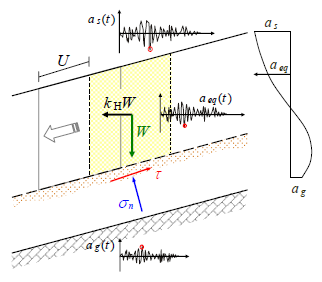
Figure 1 2D slice showing pseudostatic force kHW, after Ausilio et al.(2007)
The dimensionless parameter kH is the horizontal seismic coefficient. It represents the resultant value of the non-uniform distribution of the horizontal component of the inertia forces acting down-slope in the ground above the failure surface. The panel on the right side in Figure 1 shows how the equivalent acceleration (aeq), defined as the peak amplitude of an ‘equivalent accelerogram’ acting on the slope, might vary from the acceleration ag below the failure surface to the ground surface acceleration, as.
Slopes are not simple rigid bodies, and the peak amplitude (shown as a red dot on Figure 1) only applies instantaneously, therefore it is usual to select coefficients that provide for a lower pseudostatic force than if the peak instantaneous amplitude was applied.
There are many different approaches to the estimation of kH. Most are based on experience, or results from numerical analyses. These are discussed in NZGS (2023). Simmons (2023) discussed the practice in open pit coal mines in Australia. It is common practice to use a value of kH that is no more than 0.5 of the relevant peak ground surface acceleration.
The force diagram for a 3D limit equilibrium analysis extends Figure 1 into the in slope direction, with comparable forces and stresses acting on a vertical column overlying the slip surface. The pseudostatic force then acts in the direction of sliding that is derived by an iterative process.
With 2D analyses, the W component of the pseudostatic force is calculated using a nominal slice thickness assumed to be a unit thickness. In a 3D LE implementation, the pseudostatic force acting on the ground above the failure surface will be calculated based on the full volume of the ground above the failure surface.
It is also useful to calculate the horizontal earthquake coefficient at the point of limiting equilibrium, when the calculated factor of safety is close to 1.0. This is known as the yield coefficient ky. and can be compared with kH that was selected for the slope design.
The vertical component of an earthquake accelerogram is usually neglected in the pseudostatic method, however it is generally available as an input option for LE computer programs. It is difficult to find guidance as to selection of an appropriate vertical earthquake coefficient, kV. NZGS (2023) state “it is typical to ignore vertical acceleration”. Standards New Zealand (2004) state that the elastic site hazard spectrum for vertical loading, CV(T), for a given return period shall be given by CV(T) = 0.7C(T) where C(T) is the elastic site hazard spectrum for horizontal loading.
4. 2D VERSUS 3D LE
The early versions of TSLOPE were for 3D LE analysis only. Following feedback from users, who were unsure of the results that they were obtaining, we added the ability to carry out companion 2D slope stability analyses in the same program.
Our ongoing support of TSLOPE users has exposed us to analyses with many different types of geology and slope conditions. We have learnt that it is not always clear what the difference will be between the results of 2D and 3D LE analysis using the same slope model. Most times the 3D factor of safety is greater than 2D, especially with slopes that have constraining geometry or a failure surface along a deep weak layer. In some special cases the 3D factor of safety will be lower; a well-documented example of that is the landfill slope failure at Kettleman Hills, California (Seed et al. 1988).
Brown and Wood (2023) made a strong case for the use of 3D LE stability analysis. The paper was related to our experience with open pit mine slopes, however the same argument applies to slope engineering in non-mining applications. It is clear to us that on many occasions, a 2D slope stability analysis of a 3D problem will not provide an appropriate solution.
The benefits of 3D analysis are best shown in cases where slope reinforcement is utilised, or there are irregular point or surface loads on the slope. With 2D analysis it is difficult to model out of plane elements, and various assumptions are needed. A good example of the difference in factors of safety that result from consideration of slope reinforcement was given by Brown (2022)
5. CASE HISTORY – WAIAU TANK FARM
The November 14 2016 M 7.8 Kaikōura earthquake caused strong ground shaking at the site of the Waiau tank farm. This facility owned and operated by Hurunui District Council consisted of 25 above-ground water tanks, approximately 3.5m diameter, and 3m height, and a rectangular covered tank about 14m by 10m. The tank farm is located on a more or less flat terrace near the crest of a west-facing 53m high natural slope, with a slope angle varying between 30 – 35o to the horizontal.
Following the earthquake, more or less continuous tension cracks were observed approximately parallel to the slope crest, and up to 21m from the crest of the slope. These are shown in Figure 2
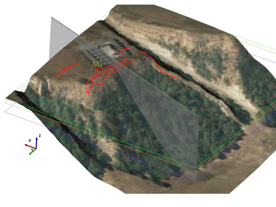
Figure 2 Waiau tank farm – TSLOPE model
Figure 2 shows an aerial photograph draped over the TSLOPE model, with red lines indicating tension crack locations, M1 drill hole location, and cross section location (grey vertical panel). The TSLOPE model also represents the 3D geological model; shallow loess soils overlying alluvial sediments (silty clayey sands, sandy gravels). At about 14.2m below ground, Tertiary age unweathered siltstone with thin layers of mudstone were encountered in drill hole M1. The unconformable contact between Tertiary age rocks and alluvium was assumed to be more or less horizontal.
The GeoNet strong motion recording site at Te Mara Farm Waiau (WTMC) is located about 5km northwest of the Waiau tank farm. As shown on Figure 3, the horizontal PGA recorded during the 2016 M 7.8 Kaikōura earthquake was 1.1g, and the vertical PGA 3.2g.
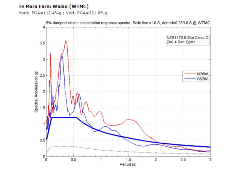 Figure 3 GeoNet strong motion data
Figure 4 shows the subsurface geology, with the Tertiary age sediments underlying the sandy gravels. The failure surface was obtained by a search for a critical surface; the slope above the failure surface is discretised into 41 equal width vertical slices. The water tanks are modelled as point loads, as shown with the purple arrows. A 10m corridor width was used to project the point loads on to the 2D section, so loads acting 5m on either side of the section line were applied.
If we follow accepted practice, then the value of kH that could reasonably be used in a 2D LE analysis of this slope would be kH = 0.4 x PGA, ie kH = 0.45. When we used kH = 0.45 in a 2D LE analysis, TSLOPE calculated a factor of safety = 1.4 (Figure 4). The relatively high factor of safety would not normally be associated with a slope that showed tension cracking as observed after the Kaikōura earthquake. This indicates that kH is either too low, or perhaps the vertical acceleration was an important consideration in slope behaviour. A further calculation was made with only horizontal ground motions to obtain ky the yield coefficient; 0.70.
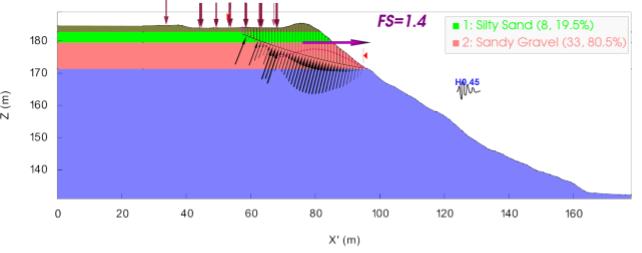
Figure 4 Waiau tank farm 2D LE output kh = 0.45
The result from a 3D LE analysis is shown on Figure 5 with a kH = 0.45 applied to the slope. The slope has been discretised into square vertical columns overlying the failure surface with width of 0.7m, the columns overlying the failure surface are shown with the dark green colour. Thirteen of the tanks and part of the covered tank overly the active columns. The ky calculated for the 3D model was 0.66.
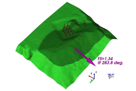
Figure 5 Waiau tank farm 3D LE output kH = 0.45 showing direction of slope failure, and factor of safety.
In this case history, the 3D LE factor of safety is less than the 2D. One of the factors that contributes to this is the way the loads from individual tanks are projected on to the 2D section, whereas in 3D the loads are in the correct location with respect to the model. Figure 5 shows the calculated slope failure direction as a bearing, 283.8o.
If we accept that we have made a reasonable estimate of kH based on the WTMC strong motion data, then there is something missing from our analysis. As suggested by the 2D analysis, we have investigated the effect of including a vertical acceleration, as represented by kV into the analysis. We have used the 3D model to find a value of kV (keeping kH constant) that would give a factor of safety of 1. In this case, as shown on Figure 6, kV is 0.34, compared with the maximum recorded vertical acceleration at WTMC of 3.21g.
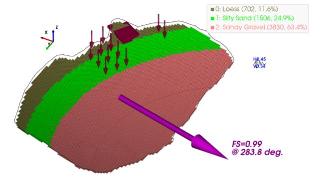
Figure 6 Waiau tank farm 3D LE output kh =0.45 kv = 0.34. Failure surface with overlying topography and layers removed. Material type shown at base of each column, with number of columns and percentage of total columns.
4. CONCLUSIONS
Pseudostatic analyses should be undertaken as part of screening for potential slope stability problems during strong earthquake shaking. If the factor of safety is calculated to be close to 1, or there is potential for loss of strength then further numerical analyses would be required to provide information on potential slope displacement.
Given the approximations and uncertainties involved with the process of pseudostatic LE analysis, we recommend that 3D models are routinely used, at least to check that there are no 3D effects that should be taken into account. We now have easy access to 3D data and software, and in most cases it is necessary to build a 3D model to inform the selection of a representative 2D section. TSLOPE is able to use 3D geographical information system data to quickly facilitate 2D slope stability analyses if they are needed to help with understanding the 3D results.
Further work is required to improve the reliability of LE analysis of slopes under strong earthquake shaking. We recommend the following:
- The New Zealand Geotechnical Society should provide comprehensive guidance on the use of 3D methods through their slope stability geotechnical guidance series of publications.
- Further work is required to assess the appropriate kH and kV that should be used with 3D LE methods. This should be informed by the application of suitable numerical codes.
- The assumption that the pseudostatic seismic force acts through the centre of gravity of the column in a 3D model should be further investigated.
- We need to identify further local examples of slope behaviour during the Kaikōura 2016 earthquake that would enable calibration as we have shown with the Waiau tank farm slope.
We should use the opportunity to improve our practice of the seismic design of slopes by using 3D LE. Confirmation of an economic slope reinforcement design may be achieved in 3D, particularly when the higher accelerations recommended by the National Seismic Hazard Model are taken into account.
REFERENCES
Ausilio, E., Silvestri, F., Tropeano, G. (2007). “Simplified relationships for estimating seismic slope stability”. Geotechnical aspects of EC8, Madrid, Spain. International Society for Soil Mechanics and Geotechnical Engineering European Regional Technical Committee ERTC12 workshop.
Brown, IR (2022) “Slope stability analysis and the new National Seismic Hazard Model”. NZ Geomechanics News, Bulletin of the New Zealand Geotechnical Society Inc. 104 58-61
Brown, IR and Wood, PJ (2023). “The case for using three-dimensional limit equilibrium stability analysis”, in PM Dight (ed.), SSIM 2023: Third International Slope Stability in Mining Conference, Australian Centre for Geomechanics, Perth, 927-938. https://doi.org/10.36487/ACG_repo/2335_63
Duncan, JM, Wright SG and Brandon TL (2014). “Soil strength and slope stability“. Second edition. ISBN 978-1-118-65165-0, John Wiley & Sons, Inc. Hoboken, New Jersey, USA. 317pp
NZGS (2023). “Slope stability geotechnical guidance series unit 1 – general guidance”. Draft. New Zealand Geotechnical Society Inc. 157pp https://www.nzgs.org/nzgs-slope-stability-guidance-draft-for-comment/
Read, J. and Stacey P. (Eds) (2009). Guidelines for open pit slope design. CSIRO Publishing, Melbourne.
Seed, R.B., Mitchell, J.K., and Seed, H.B. (1988). “Slope stability failure investigation: Landfill Unit B-19, Phase 1-A, Kettleman Hills, California”. University of California, Berkeley Department of Civil Engineering Report No. UCB/GT/88-01. 96pp
Simmons, J.V. (2023). “Earthquakes are exciting for coal miners too”. Australian Earthquake Engineering Society 2023 National Conference, Brisbane, Queensland, Australia.
Spencer, E. (1967). “A method of analysis of the stability of embankments assuming parallel inter-slice forces” Géotechnique, 17 11-26
Standards New Zealand (2004). “NZS1170.5: Structural Design Actions. Part 5: Earthquake Actions ‐ New Zealand“. Standards New Zealand, Wellington, 76pp. https://www.standards.govt.nz/sponsored-standards/building-standards/NZS1170-5
TAGA Engineering Software Ltd. TSLOPE version 2.3 https://tagasoft.com
Wyllie, D.C. (2017). Rock slope engineering: civil applications. Fifth edition. ISBN 978-1-498-78627-0 Taylor & Francis, CRC Press, Boca Raton, Florida, USA. 568pp
ACKNOWLEDGEMENTS
Mason Reed of Fraser Thomas Limited, consulting engineers, introduced Ian Brown to the Waiau tank farm case history.
The paper has benefited from discussions with and review by Dr Tam Larkin.

